NeurIPS Learn to Move Competition

Over the past four months I took part in the Learn to Move: Walk Around challenge, one of the challenges among the NeurIPS 2019 Competitions Tracks. The goal of the competition is to develop human-level versatile locomotion controllers, a grand challenge in biomechanics, neuroscience, and robotics; this year specifically, the main task was to develop a controller for a 3D human musculoskeletal simulation model to walk or run following velocity commands. In this post, I will follow my progression through the competition, what I tried that worked and didn’t work, and what my thinking was in approaching some of the problems I ran into. I am sharing my code here. I finished third in round 1 and sixth in round 2 of the competition among 307 participants (leaderboard).

This post is organized as follows:

1. TL/DR my final approach and model
2. Introduction to the challenge and simulation environment
3. Preparation
4. Getting things going — initial considerations
5. Speeding things up — exploration algorithms
6. Producing a realistic gait — reward augmentation and gait symmetry
7. Improving action selection — policy modeling and action selection
8. Conclusion

TL/DR my final approach and model:

My final submission used the following:

• learning algorithm — Soft Actor Critic (ref paper) with automatic/learnable entropy adjustment (ref paper) and a BNAF normalizing flow (ref paper) on top of the policy. The networks used were all feed-forward: 2x128 (# layers x # hidden units) policy network + 3x66 BNAF on top, and 2x256 for the value and Q networks. Activations throughout were ReLUs.
• exploration algorithm — based on Self-supervised Exploration via Disagreement (ref paper), I added an exploration bonus equal to the variance of the predicted next states computed over 5 state predictor models and along the predicted state vectors (i.e. reward is high for states the predictors cannot model well (new states, where they disagree) and for diverse state vectors (away from e.g. symmetrically standing motionless)). The state predictor networks were each 2x64 and operated only on the pose information from the state space.
• best action selection — since I had the trained state predictor models for exploration, I used them to select a best action by first sampling 10 actions from the policy, then predicting the next state using the state predictor models (pose only; recall that the state predictors operate on pose information only), then computing my reward from this hypothetical (s, a, s’) transition, and finally selecting the action yielding the best reward.
• state space transformations — I pooled the 2x11x11 velocity target field into a 2x3 matrix for the positions immediately adjacent to the agent in the x and y directions - this seemed justified for motion planning since a/ this is an MDP, b/ the agent cannot reach beyond the positions immediately adjacent and c/ the mapping is continuous so goal distance varies smoothly. I left the pose and limbs information unchanged.
• environment transformations — I used the following sequence of environmental wrappers:
  • random pose initiation (initiates the agent in a mid-stride pose from a realistic gait; I manually tweaked the parameter ranges to produce credible snapshots of a walking motion),
  • action augmentation (transforms the [-1,1] output of the policy to the [0,1] input to the simulator),
  • velocity target pooling (transforms the 2x11x11 velocity target around the agent to a 2x3 target for the positions immediately adjacent to the agent in the x and y directions),
  • reward augmentation (added rewards functions for the velocity target distance, x-velocity, y-velocity, yaw target, pose components pitch and roll, and pelvis height),
  • frame skipping (repeated each action 4 times).
• training — I trained for almost 270k steps over 4 parallel environments.

This setup produced the following agent:

Introduction to the challenge and simulation environment

The Learn to Move: Walk Around challenge provides a human musculoskeletal model and a physics-based simulation environment, OpenSim, to develop a controller for a physiologically plausible 3D human model to walk or run following velocity commands. Full documentation on the simulation environment is available here. Below is the output of the simulation — 3D human musculoskeletal model (right) and target velocity maps (global map: top-left; local map: bottom-left). The evaluation rewards for round 1 were designed to be high when the human model locomotes at desired velocities (indicated as the vector field in the local velocity map) with minimum effort; the round 2 rewards included a target bonus if the human model stays for 2-4 seconds near the target (where the velocity target is 0; also indicated as the center of the concentric circles the global velocity map) and extended the simulation time from 1000 to 5000 time steps (round 2 rewards are described in detail below).

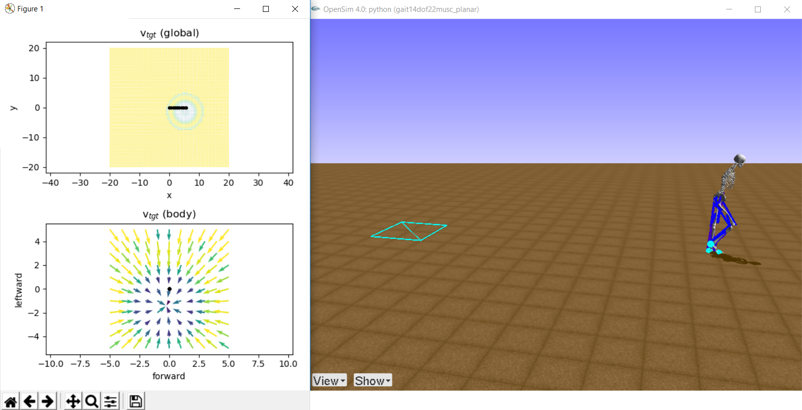
State space — the state space includes a 2x11x11 target velocity map and a 97 dimensional body state vector comprising continuous values for pelvis state (height, pitch, roll, and 6 velocity parameters), ground reaction forces (3 for each foot), joint angles and velocities (4 joints for each leg), and muscle states (11 muscles on each leg with 3 parameters for each muscle - fiber force, length, and velocity).

Action space — the action space represents muscle activations of the 22 muscles (11 for each leg), continuous in the [0, 1] interval.

An agent with random muscle activations yields the following:

Preparation

RL background. My own goal in participating in the challenge was to dive deeper in reinforcement learning. A few great resources I used in preparation and to source ideas were:

• Sergey Levine’s Deep RL class at Berkeley CS-294-112. Going through the videos, slides and working through the homeworks gives a solid background on RL (imitation learning, DQN, PPO, SAC, model-based RL, meta-learning, exploration).
• Spinning Up in Deep RL by OpenAI. This has slim implementations of the main deep RL algorithms and a great reference list of key RL papers.
• Deep RL Bootcamp from 2017. Though a bit old, this has good reviews of some of the state of the art algorithms.

Previous competitions. I reviewed the papers summarizing the challenge solutions to previous year Learn to Move competitions (here for 2018 and here for 2017) in order to get a sense for the algorithms used and general approaches to the problem. Previous competitions were quite different: in 2017, 2D locomotion (i.e. agent cannot fall sideways); in 2018, 3D prosthetic leg locomotion in which the agent had to maintain different target velocities (velocity target was strictly ahead and there was no requirement to stop and restart or change direction). Participants in both competitions had used predominantly model-free RL, mostly parallelized DDPG and a few PPO implementations with various reward augmentation strategies.

Testbed. I needed a setup to iterate quickly, save and load experiments, compare and plot results. I looked into OpenAi Baselines, Ray, garage (previously Berkeley’s RLLab), and dopamine. I borrowed the Baselines setup (run entrypoint, vectorized environments, gym environment wrappers, algorithm core modules) and built a slimmer/simpler implementation for both OpenAI Gym/Mujoco and OpenSim. I ran HalfCheetah baseline tests whenever I tried new features and algorithms, since this environment has a small state and action space and iterating in it is very fast. I ran some tests in the Humanoid environment as well, which is conceptually close to OpenSim and faster than OpenSim, however it uses joint torques for control and the action space extends to the torso. As a result, experiments on Humanoid do not translate to OpenSim easily, outweighing the speed benefit.

Getting things going — initial considerations

I started focused on learning a simple agent quickly. From there I could add complexity and hopefully still iterate quickly. I simplified the models and the environment and benchmarked learning algorithms to arrive at good base-case functioning algorithm.

The MDP. The OpenSim environment produces positions, velocities, and accelerations, which completely define the physical state of the agent at any given time without reference to past states. In principle, the agent can determine the next action without keeping track of the prior trajectory. This led me to use feed-forward networks (instead of recurrent with multistep loss). If, in addition, we focus the reward (more on this later) on incentivizing gait stability, velocity and turning goals, i.e. the reward is not episode dependent but transition dependent, then we should be right in the sweet spot of off-policy learning from a memory buffer. Off-policy algorithms was also very helpful since they are much more sample efficient than on-policy ones and I ran experiments predominantly on my laptop.

Selecting the learning algorithm. I implemented TD3, DDPG, and SAC. TD3 performed much worse, so after some initial tests I abandoned TD3. I used a slightly different implementation of DDPG (similar to the one benchmarked in the TD3 paper - no state vector centering, no reward scaling). Using SAC out of the box did not work - SAC is very sensitive to the alpha entropy weight parameter and OpenSim is too slow to tune alpha meaningfully. Once I made alpha learnable, SAC showed much faster learning than DDPG on the 3d human model. Interestingly SAC and DDPG exhibited very different walking patterns over the course of learning, at different number of training steps at every environmental step. My favorite:

SAC on 2d model after 60k training steps:

DDPG on 2d model after 80k training steps (20 training updates / environment update):

Simplifying the environment. The OpenSim environment provides the options to 1/ use a 2D or 3D model (the agent can’t fall sideways in a 2D environment) and 2/ position the velocity target strictly ahead, in the 180 degree forward view of the agent or anywhere in the 360 degrees around the agent. Learning in 2D is much faster than learning in 3D, so to benchmark my initial approaches I used a 2D simulation and a strictly-ahead velocity target.

Simplifying the state space. I tried making the state space smaller in order to speed up learning. I tried using subsets of the state vector for policy learning (e.g. pose information only), but that led to learning plateauing early. I also tried using a more compact representation of the velocity target field. OpenSim provides a 2x11x11 agent-centered velocity targets grid of the x and y coordinates, updated with every environment step. The generated velocity target vector field looks as follows:



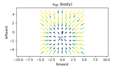
The agent, however, can only reach within a radius of 1 making the velocity target map beyond that uninformative. I decided to pool the 2x11x11 velocity target vector field into two 3-dim vectors for the x and y directions - I subsampled every other position in the 11x11 maps, followed by 2x2 average pooling with stride 2 (I tried convolving a moving average window but that led to some distortions). This quantized the y direction to 3 locomotion controls: straight, straight and to the left, and straight and to the right. The x direction, in turn, quantized to 3 controls: target ahead of agent, target on top of agent, and target behind agent. My final agent orientation looked as follows: 

I tied various parametrizations of the velocity target map in the y direction specifying how the agent should turn — e.g. 1/ one-hot direction vectors quantized to 3, 5, and 7 angles around the agent; and 2/ continuous yaw targets specifying the difference between current yaw and the yaw needed to face the target. I also tried various parametrizations of the velocity target map in the x direction specifying the speed and distance the agent needs to move in the forward direction — e.g. 1/ inverse of the Euclidean distance to target, 2/ x-velocity target only without distance, 3/ one-hot vector stop and go with fixed forward velocity target, 4/ various quantizations of the target x velocity. This search for the right parametrization went on until the end of the competition, and in the end, I was not able to meaningfully stop and hover the agent over the target.

Speeding things up — exploration algorithms

My initial experiments showed quickly that I needed to speed up learning and my ability to iterate experiments. The OpenSim simulator was orders of magnitude slower than the Humanoid environment in Gym/Mujoco, and human poses at the limits of the simulator ranges slowed it orders of magnitude on top of that (e.g. body parts other than feet touching the ground, when agent falls). I had already done several things to improve speed — I lowered the simulator integration accuracy (integrating the action input into the dynamics model to produce the next state); I tried increasing the stepsize (simulator steps in between action inputs), though this led to unrealistic motion); I had vectorized environments and was running 4-8 environments in parallel; I had parallelized DDPG using MPI (SAC, on the other hand, is not parallelizable, though I tried it anyways, and indeed it didn’t work).

Two factors impacted speed and added to the difficulty of the competition:

1. The state space is large and continuous — as an example, going from 2D human model to 3D human model meant going from 20k steps to 100k training steps before seeing results (equivalently, for a small model size and slimmer algorithm, this meant 2 hours -> 10 hours on a laptop).
2. A long sequence of actions is required to perform a step — this meant that exploration is temporally connected. Specifically, a single gait cycle was about 25 steps at a frame skip of 4 steps (i.e. each action repeated to the simulator 4 times); thus, decisions to explore early in the gait cycle determined the possible states the agent could explore later in the same gait cycle. This is different from the nature of the physics-based MDP — given the current state, the agent still has all the physical information needed to decide the next action; learning the optimal policy to generate this next action, however, has to do with exploration and exploration is over a continuous state space over ~ 25 time steps, and this is difficult.

A principled way to improve learning speed was a better exploration strategy. In the current regime, simply doing uniform epsilon-greedy exploration was both inefficient, given the large and continuous state space, and time-independent, such that actions in a sequences are explored independent of each other contrary to the nature of the task. I implemented several algorithms to improve exploration:

1. Exploration via disagreement — this was inspired by Self-supervised Exploration via Disagreement and the idea is that several (I used 5) state predictors model the next state given the current state and policy action. The variance among the state predictors and over the predicted next state vectors, is added to the rewards as an exploration bonus. This means that if we can predict the next state well and the predictors agree, variance and therefore the reward bonus is low; conversely if we can’t model the next state well, variance is high, the reward bonus is high and the agent is pushed to explore the state we can’t yet model well. On the other hand, variance is also taken over the state vector dimension, incentivizing exploration of diverse state vectors (e.g. left-right leg mid-stride having opposite signs is higher variance than standing and having legs in same position). I found this form of exploration significantly improved sample efficiency in both the HalfCheetah test task, when compared to other strategies, and the Learn to Walk task. It also outperformed the other exploration strategies. In order to make my implementation more efficient, I decided to model only the pose information of the state space. This way, I could use smaller networks for each of the state predictors (in the end, since only the variance matters, the size of the predicted state space is not relevant).
2. Ensemble with randomized prior functions — this was inspired by Deep Exploration via Randomized Value Functions and its successor Randomized Prior Functions for Deep Reinforcement Learning which I implemented. The idea here is to ensemble several separate models, each trained on a subset of the data, which together approximate a posterior. In the successor paper, the ensemble is improved by adding a random but fixed prior functions to each of its members. In practice, I added a random and non-trainable prior to the value and Q networks in SAC (and only Q network in DDPG) and trained each member of the ensemble on separate samples from the same replay buffer in order to improve speed and memory footprint. When acting in the environment, since I vectorized 4-8 environments in parallel, I re-sampled the acting policy head ranging from 20 steps (a single stepping motion) to 1000 steps (length of an episode, though again, several environments in parallel do not all run concurrent episodes). In the end this strategy showed poorer sample efficiency than SAC alone on both OpenSim and HalfCheetah.
3. Exemplar models — this was inspired by EX2: Exploration with Exemplar Models for Deep Reinforcement Learning. The idea here is that certain states are representative of the walking motion and we want to reward the agent for staying close to these ‘exemplar’ states. My implementation of the exemplar algorithm is quite different from the original paper — instead of learning what an exemplar states is by training a VAE, I specify the exemplar states via a dictionary sampled at initialization by randomly resetting the initial pose from a range of parameters, for which the pose resembles a snapshot of a natural walking motion (in OpenSim the initial pose is specified by 12 parameters vs. the 97 dimensional full state space, which makes hand crafting initialization parameters easier). I then include as exploration penalty the L2 distance from the current state and the normalized mean exemplar state — the result is that states from a walking trajectory would be close to the dictionary mean and incur a small penalty, while states, where for example the agent is falling sideways, would be far from the dictionary mean and thus penalized more. This also unfortunately underperformed the other approaches. If I had more time with the competition, I would have tried to better align the current state with the closest dictionary state instead of using the mean.

There is a body of work on distributional RL. It is important to make the distinction, however, that we are exploring unknown and not stochastic outcomes. We do not need a distribution over the realized value under stochastic outcomes, but rather need to explore the distribution brought on by the uncertainty in the optimal value/Q functions (for extended discussion, ref [Deep Exploration via Randomized Value Functions]).

There is also body of work on count-based and intrinsic motivation exploration, involving density models (ref Unifying Count-Based Exploration and Intrinsic Motivation and #Exploration: A Study of Count-Based Exploration for Deep Reinforcement Learning), which is effectively captured by the exploration via disagreement I described above. In the end, I settled on exploration via disagreement and shifted focused to different policy representations, improving the parametrization of the velocity target, and augmenting the reward function.

Producing a realistic gait — reward augmentation and gait symmetry

As RL goes, one can spend all their time tweaking the reward function. So did I. I kept coming back over and over again to the reward function and the state representation (specifically velocity target map) going into that reward function. The agent had to walk to a target at a desired velocity, stop at the target, then after 2-4 seconds the target would change and we repeat. In general, I made a distinction between high-level control (go, stop, turn) and low-level control (walk/gait actions to simply walk forward), so I needed a state representation with appropriate rewards that can allow for both. (I did experiment with hierarchical RL, see below). High-level control proved much more difficult than low-level control. Correspondingly, I spent almost all my time tweaking the reward function on the goals and control items below.

My final reward function is a sum of the components below. I have left all the coefficients as the final numbers I used (a plethora of greeks would make the below read even more unintelligible). I ran experiments to determine the correct scale for each and used several other functional variants before settling on tanh’s.

Reward function components:

• goals — reward the agent for approaching the velocity target by facing it ahead ($y_{(1)}$) and in front ($x_{(1)}$) and for staying close to the velocity target field center.

$$\begin{aligned} \text{velocity target distance} & = \max(0, \tanh (\frac{1}{\max (0.1, d)} - 0.5)), \; \text{where} \; d = \sqrt{x_{(1)}^2 + y_{(1)}^2} \\ \text{velocity target goal} & = 5 * \mathbb{I}(d < 0.3), \; \text{with $d$ same as above} \end{aligned}$$

• control — reward high x velocity when away from target and low when near target; reward low y velocity; reward yaw (turning) towards the minimum y velocity target (recall objective is to find the velocity field center/sink).

$$\begin{aligned} \text{x velocity} & = \begin{cases} 3 * \tanh (dx), & d > 0.3 \; \text{with $d$ same as above} \\ 2 * (1 - \tanh(5dx)^2), & d \le 0.3 \end{cases} \\ \text{y velocity} & = - 2 * \tanh (2*dy)^2 \\ \text{yaw} & = 2 * (1 - \tanh (100(\Delta yaw - \Delta yaw_{tgt}))^2), \\ & \quad \; \text{where $\Delta yaw = yaw_{t+1} - yaw_{t}$} \\ & \quad \; \text{and $\Delta yaw_{tgt} = 0.025 * ([1, 0, -1] \cdot y_{vtgt})$} \\ & \quad \quad \quad \text{with $y_{vtgt}$ 3-d one-hot of the $y_{vtgt}$ argmin} \end{aligned}$$

• stability — reward stable pitch and roll by penalizing reinforcing loops (e.g. when agent is falling forward, pitch is (+); if the pitch derivative $\partial pitch$ is (-) the agent is counteracting the pitch, if $\partial pitch$ is (+) is reinforcing the pitch and will continue to fall forward. Thus penalize if the metric and its derivative have the same sign).

$$\begin{aligned} \text{pitch} & = - \max (0, \; pitch * \partial pitch) \\ \text{roll} & = - \max (0, \; roll * \partial roll) \\ \text{pelvis height} & = - 5 * \mathbb{I}(\text{height} \le 0.7) \end{aligned}$$

• OpenSim environment round 2 evaluation rewards (provided by the organizers) — reward being alive; reward making new steps (defined by alternating left/right foot contact with ground); penalize deviations from target velocity; penalize effort; reward task success if stayed enough at the target.

$$\begin{aligned} \text{alive} & = 0.1 * \Delta t , \; \text{where $\Delta t$ is environment timestep} \\ \text{footstep} & = 10 * (\sum_i{\Delta t_i}) * \mathbb{I} (new \; step = true) \\ \text{footstep velocity} & = - \; 3 * \lVert \sum_i{\Delta v_i * \Delta t_i} \rVert, \; \text{where $\Delta v_i = v_{body} - v_{tgt}$} \rvert_{t=t_i} \\ \text{footstep effort} & = - \sum_i{(\lVert muscle \; activations \rVert_i ^2 * \Delta t_i )} \\ \text{task bonus} & = 500, \; \text{when on top of velocity target field center for 2-4s} \end{aligned}$$

In addition to the above, several approaches proved unsuccessful:

• using ground reaction forces for each foot to incentivize lifting feet and stepping
• using vertical (z) velocity to incentivize bending the knee
• using pose similarity to incentivize return to pose at initialization (this could have worked better if I had access to dense trajectories and done imitation learning; the organizers did provide real gait trajectories, but I did not have time to experiment in this direction)

Gait symmetry / covariance. Symmetry is an important feature of what we would qualify as a normal gait. Specifically, locomotion is left-right (sagittal plane) symmetric and I tried to use/reward this symmetry in 3 separate approaches - adding a symmetric action loss term, using a symmetric memory buffer, and shrinking the policy to act on a single leg. Before explaining each approach, below is a video of an agent trained to 275k steps and the plot of the its action covariance matrix for the 22 muscle activations (the gait itself is not exactly symmetric but the covariance structure within each leg and between the legs is evident):

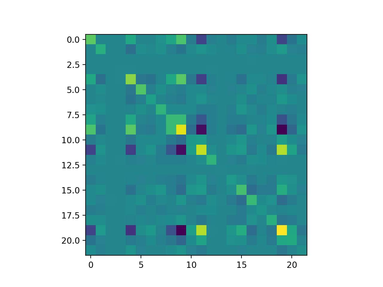
Action Covariance plot:  We can see a 2x2 block structure with the blocks on the diagonal blocks reflecting the right and left legs. Each diagonal block has itself a diagonal bottom right block revealing the covariance of knee flexor and ankle extensor muscle activations. For the specific muscle sequence on each leg see the official docs here.

My attempts at using symmetry in more detail were as follows:

1. symmetric action loss function — inspired by Learning Symmetric and Low-Energy Locomotion, this encourages the policy to output symmetric actions by adding an L2 loss term between the policy action and a ‘symmetry mirrored’ action. The symmetric mirrored action is produced by first left-right mirroring the state, then using the policy to act on the mirrored state, and finally left-right mirroring the action produced by the policy. If the policy acts symmetrically this loss term component will be zero. I found that adding this symmetry loss term helped produce a more symmetric policy, though, tweaking the scaling coefficient of the loss term was difficult and had a significant impact on the speed of learning.
2. symmetric memory — in this approach, each (s, a, s’, r) tuple stored in the memory buffer was saved once as is and once mirrored along its left-right symmetry. In theory the agent would learn from symmetrical experiences encouraging the policy to produce symmetric actions. In practice, however, the agent failed to learn. The issue appeared to be that while a gait is symmetric over time (e.g. left steps follow right steps), inside a gait cycle the agent has to break symmetry in order to move forward. This proved challenging to policy learning as it could require observing a full gait cycle before calculating rewards or adding experience to memory. Waiting for a full gait cycle was particularly difficult using off-policy algorithms, which I was using, so I dropped the idea.
3. single-leg policy — under this approach the policy only models half of the action space (i.e. a single leg) and is called twice to get left and right leg actions (I tried this with and without conditioning on the previous-leg action). The idea was that controlling a smaller action space should be easier to learn and that, in a symmetric gait, moving the right leg forward given where the left leg is, is no different than moving the left leg given where the right is; thus we only need to control one leg and condition on the state plus action for the other leg. I also tried removing the conditioning and instead running the single leg policy twice on every state input for each leg. This produced interesting knee-bending behaviors which other policies generally struggled with (video below). In the end, this approach to policy parametrization did not perform well.

Single leg policy at 2k training steps:

SAC baseline at 2k training steps:

Improving action selection — policy modeling and action selection

In the second half of the competition, I tried several strategies to improve the policy and action selection. I have separated those in what worked and what didn’t work below.

What worked:

• normalizing flow on top of the policy — normalizing flows are a technique used to model probability density (ref Glow: Generative Flow with Invertible 1x1 Convolutions or Masked Autoregressive Flow for Density Estimation and my Github repo on flows here). Specifically, a flow is a series of bijective transformations used to transform a base probability distribution into a richer, multimodal distribution - e.g. a standard normal N(0,1) can be transformed to a multimodal distribution or the distribution over images of faces. In a way, a normalizing flow is able to better capture the covariance of the data, even when the underlying base distribution on its own cannot. In this second half of the competition, I had settled on SAC, in which the policy outputted a Normal distribution with diagonal covariance. Adding a normalizing flow on top of the distribution produced by the policy, thus, allowed me to better capture the covariance among the different muscle activations (e.g. knee bend associated with lifting the foot). In the end, this sped up learning and produced more realistic walking motion. I used Block Neural Autoregressive Flow (BNAF for short, ref paper), which was the most flexible and fastest-to-learn flow that I had used.
• model-based action selection — I decided to borrow a technique for action selection from model-based RL, namely n-step lookahead. I blended this with my off-policy algorithm into a hybrid model-free + model-based approach. Specifically, at each environmental step, m actions are sampled from the policy. The trained state predictor models used in the exploration algorithm serve as a dynamics function to produce a predicted next state (in earlier iterations I used the state predictors on pose information only, which forced me to use distillation on the policy in order to act only on pose information in the model-based rollouts). The (state, action, next_state) tuple is then passed through the reward function to calculate predicted reward. The policy is then resampled on the batch of m predicted next states. This policy resampling is repeated n times, hence n-step lookahead. Finally, the first action with best aggregate reward over the trajectory is selected and inputed to the environment. For the n-step lookahead I used n=5 and m=32. This strategy did speed up learning compared to the SAC baseline (in terms of sample efficiency, though at the expense of slower runtime), however, was only slightly better than SAC + BNAF and disagreement exploration altogether. Much of the above was inspired in part by (though deviated much from) Model-Based Value Estimation for Efficient Model-Free Reinforcement Learning, When to Trust Your Model: Model-Based Policy Optimization, and Continuous Deep Q-Learning with Model-based Acceleration.
• curriculum learning — I used two general approaches towards curriculum learning: 1/ schedule around the initialization parameters, and 2/ schedule around the task complexity (an example approach in the domain of human locomotion can be found in Learning Symmetric and Low-Energy Locomotion). Around initialization parameters, I used realistic snap-shot poses of a walking motion as initial pose for each episode, as described earlier. At test time, the agent started from a ‘zero-pose’ of standing straight up with feet aligned (as an aside, learning from this starting point was much slower), so I annealed the random initialization pose into this ‘zero-pose’, which helped the agent at test time. Around task-complexity scheduling, I ran a few experiments learning a curriculum, involving learning forward, fixed-speed locomotion first, then introducing yaw rewards for turning towards the target and stopping rewards to pause on the target. It took 2-3 days to learn each model and my final result was not any different then end-to-end learning. In hindsight, a better path over complexifying the task could have worked much better. I tried running idealized scenarios, where, for example, the velocity target field focuses on only a fixed number of places and learning a curriculum from there, though there was too little time to try this more expansively.

What didn’t work:

• auxiliary rewards — the distinction I was making between high-level control (stop, go, turn) and low-level control (stepping motion, stability) led me to experiment with splitting the total reward from a scalar into a vector with components for goal, velocity, and stability. I would then learn separate policy heads on top of a shared state encoder, and combine everything into the loss function. This was more fully developed in the Reinforcement Learning with Unsupervised Auxiliary Tasks. Specifically, the authors compose auxiliary tasks with separate rewards and use separate policy heads for control, sharing some parameters, thus forcing the agent to balance improving performance among the main task and the auxiliary tasks. Implementing this on top of SAC proved more involved. In the end, I was not able to make this work. Given more time, though, I still think it is a promising approach for this task.
• hierarchical RL — the same distinction between high- and low-level control led me to hierarchical RL. One of the approaches I pursued was inspired by the FeUdal Networks for Hierarchical Reinforcement Learning and The Option-Critic Architecture, identifying the ‘worker’ with the low level walking controller and the ‘manager’ with the high level goal controller. The worker receives the body state vector at every environment step, while the manager receives the body state vector, plus goal and velocity target information at every 10 environment steps. I experimented with various reward functions for the two controllers. One problem I faced, which I didn’t have time to explore further, was that the reward functions for the two controllers may deviate - in a sense that maximizing one could mean minimizing the other. As an example, in HalfCheetah, the reward function has two components - speed and stability; in a successful policy, the high total reward is driven by the large velocity reward, while the stability reward is consistently negative. This means that a hypothetical hierarchical controller splitting the reward function into velocity and stability components would have to minimize one and maximize the other in order to maximize the total reward. The relationship between the manager and worker could be more subtle and complex. The authors’ solution was that the manager has access to all rewards and thus implicitly learn to trade off high- and low-level control. My experiments with this on HalfCheetah underperformed my baseline so I dropped it.
• n-step returns — as I researched hierarchical RL, I came across a recent paper from UC Berkeley Why Does Hierarchy (Sometimes) Work So Well in Reinforcement Learning?, which breaks down a set of hypotheses behind hierarchical RL and tests them. Among those hypotheses are temporarily extended training and exploration - specifically, 1/ the high-level controller observes and acts over multiple steps of the environment, episodes are effectively shorter, rewards propagate faster, and learning is faster, and 2/ exploration at the high-level is correlated over time steps thus more efficient (and more fitting to the Learn to Walk task). The authors conclude that n-step returns could achieve the same temporal extension during training and that ‘switching ensembles’ (effectively my implementation of Deep Exploration via Bootstrapped DQN) could achieve the same temporal exploration. I implemented n-step returns but it underperformed both on OpenSim and HalfCheetah, which was also my experience with the deep exploration method. I dropped n-step returns and completely dropped hierarchical RL as well.

Conclusion

The Learn to Move tasks was an good and interesting competition. Compared to previous years’ leaderboards, scores this year were much more spread. In my case, different algorithms/approaches made a big difference for the score and small tweaks to hyperparameters left it almost unchanged. This pushed me, and I assume equally others, to try to solve the task rather than run endless sensitivities and tuning to squeeze out performance from a largely fixed model. RL aside for a moment, it was interesting to think about the requirements for human locomotion, what are sufficient and necessary conditions, and what reward structure produces different gaits (e.g. just think about why we bend our knees).

I learned a lot from the competition. First, it was a worthwhile dive into deep RL. I touched on many major aspects of the field - model-free control, off-policy learning, exploration, model-based dynamics and action selection, curriculum learning, imitation learning, reward shaping, etc. A lot of public RL code is custom and difficult to reuse, so this forced me to implement most of the ideas I tried from scratch. This itself was a great and fun exercise. In addition, much of the published work in RL is far from cookie-cutter, so generalizing an approach in a paper to OpenSim and the Learn to Move task was not a given. Second, it was a worthwhile exercise in setting up and managing multiple experiments. This was different from my previous work in deep learning, where concurrent experiments most often meant architecture search, hyperparameter tuning, or data augmentation. Here, I was searching for the right learning and exploration algorithms, models, hyperparameters, state representation, reward function, initialization curriculum, etc. - all of which were interrelated and, given the time it took to run a single experiment in OpenSim, slow to test exhaustively by any means.

In the end, I was far behind the leaders. My greatest hurdle was finding a meaningful state representation of the velocity target map and controlling stopping and going behavior. I did some (too few) experiments on toy scenarios where I could test specific aspects of the reward function or learning progression. In hindsight, I should have tried to isolate the behaviors and idealized scenarios I was seeking to solve and stayed with these toy environments longer, until I have a firmer grasp of why the agent is performing in a certain way. That’s for the next time.